
OLAP databases - A Primer
OLAP vs OLTP and the evolution of OLAP

Developer who sees beyond the hype
We all are aware on the traditional relational databases such as MySQL, Oracle, Postgres etc. These are what we use daily for daily interaction through our CRUD (Create, Read, Update and Delete) apps. Whilst these are immensely useful and needful technology; there has been a new type of databases that are for generating insights on the transactions that have occurred in OLTP/traditional relational databases. That is where OLAP databases come in; they provide a historical context on the normal business operations.
OLTP can act as a analytical source of truth as is, but when you scale today's data, it becomes a complex system with huge amounts of data. These can lead to queries taking hours to run. Also, scalability and high availability at that scale becomes difficult, if a single-node architecture is used.
OLAP has gone through various iterations over the decades in order to solve the problem of complex queries, high availability, good querying performance.
Firstly, we'll look into the Shared-* architectures (Shared Disk vs Shared Nothing Architecture)
Shared Architectures
Sharing means three things: Compute, Memory and Storage
Shared-Everything Architecture
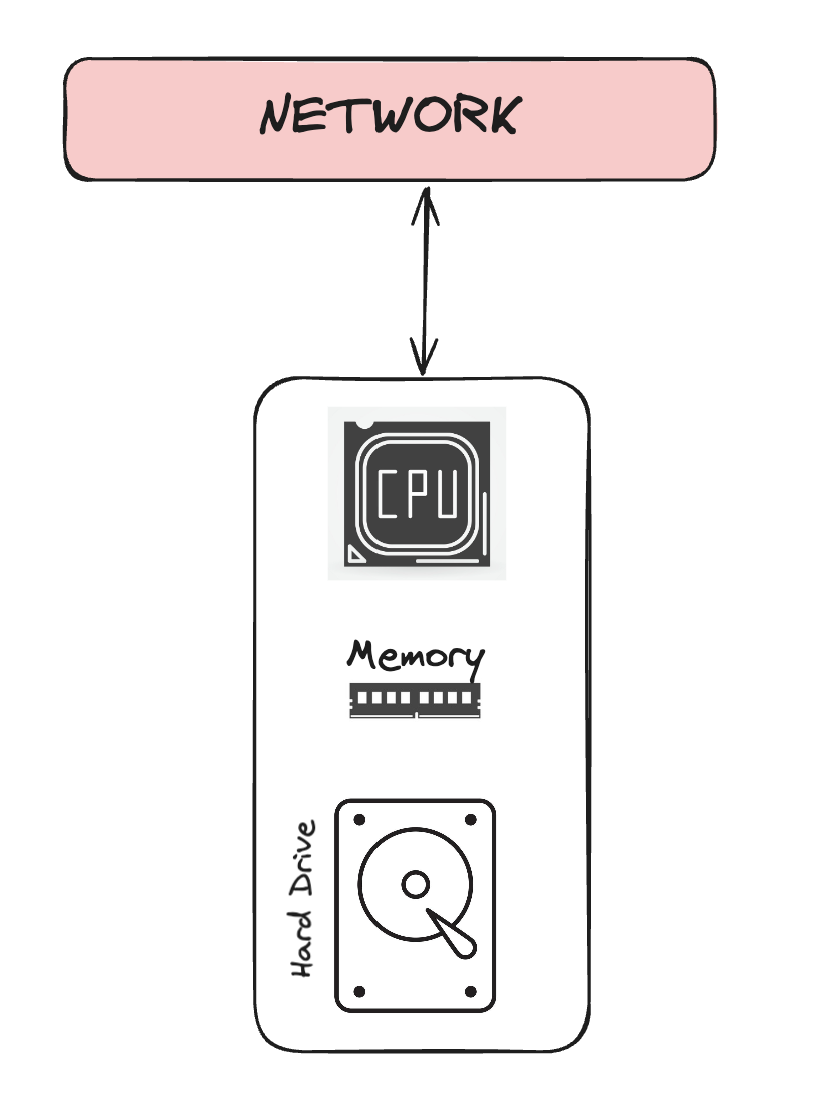
This is a single node architecture. Everything is shared. Example would be a UNIX OS where all things is in same machine. This is great for co-location but not good for fault tolerance and performance. Single server means single point of failure, hence no fault tolerance. All data in one machine without partitioning means performance degradation with larger data.
Shared-Disk and Shared-Nothing provides some improvements in each of the criteria.
Shared-Nothing Architecture
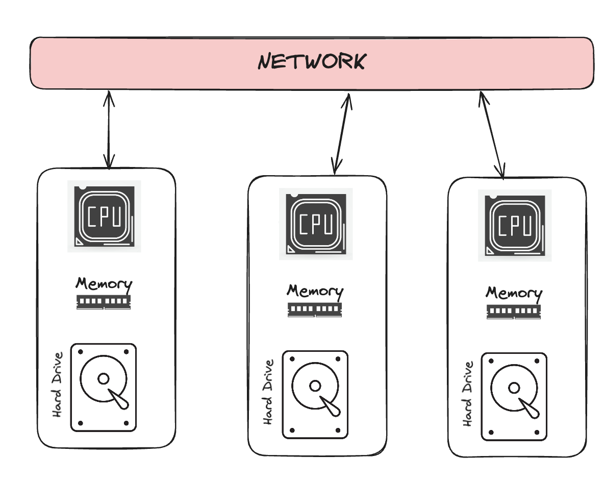
Each Database node shares:
CPU
Memory
Storage
These Nodes talk to each other via a shared Network. Data is split/partitioned into subsets across the nodes.
Data is fetched via POSIX API [?]
Shared-Nothing is harder to scale data capacity due to tightly-coupled storage layer. But these can have better performance due to co-location of data and compute per instance.
Shared-Disk Architecture
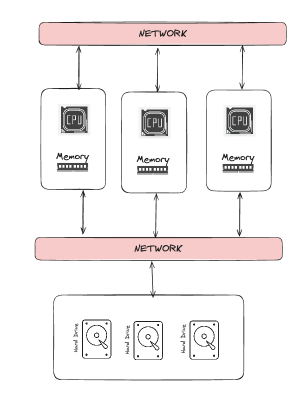
Each Database node shares the compute layer:
CPU
Memory
The storage layer is decoupled and nodes can talk to the storage and with each other via Network layer(s).
Data is fetched via userspace API instead of a POSIX API such as fread(0)
Shared-Disk is easier to scale data capacity due to loosely-coupled storage layer. But these can have lead to higher computing resources utilization as the data needs to be moved from storage -> compute layer and perform filter at compute layer.
Row Oriented vs Column Oriented Stores
One of key difference between OLAP and OLTP databases is how the data is stored.
In OLTP, as the data is queried based on IDs (Mostly), a single row/tuple is mainly the querying layer.
In OLAP, mostly the querying is based on Columns with several GROUPBY statements.
Hence, the traditional databases such as MySQL, Oracle, Postgres used row-oriented storage whilst OLAP databases such as MonetDB, Vertica use Column-oriented stores.
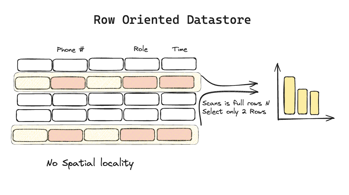
Row-Oriented Store
Here data is stored as rows at storage layer.
For example
|ID| Name | Department |Role|
|10|Ram   | Devops     |SDE1|
|20|Sam   | Security   |SDE2|
|30|Aditi |Software Dev|SDE3|
In a traditional DB, ID#20 would be a query to get information on Sam. There could be some JOINs but the data in most cases would be for a particular row.
Row-oriented can be changed to column-oriented (as early OLAPs did by forking Postgres to be column-oriented); but these have the baggage of row-oriented metadata which does not bring major performance for Analytical workloads
Some implementation that were done to move row-oriented to column oriented-database
Improving Row-oriented datastore to become Column-oriented
| What | How | Disadvantage |
| Vertical Partitioning | - Connect column by adding position attribute to every column. | - Row stores have heavy metadata info for every row. This increases space as this is not needed fro column scans |
| Index-only scans | B+Tree index for every column | Index scan for every read can be slower than traditional heap-file scan in vertical partitioning |
| Materialized Views | Create a temporary data fro faster access | Changing business need might make Materialized view largely irrelevant. |
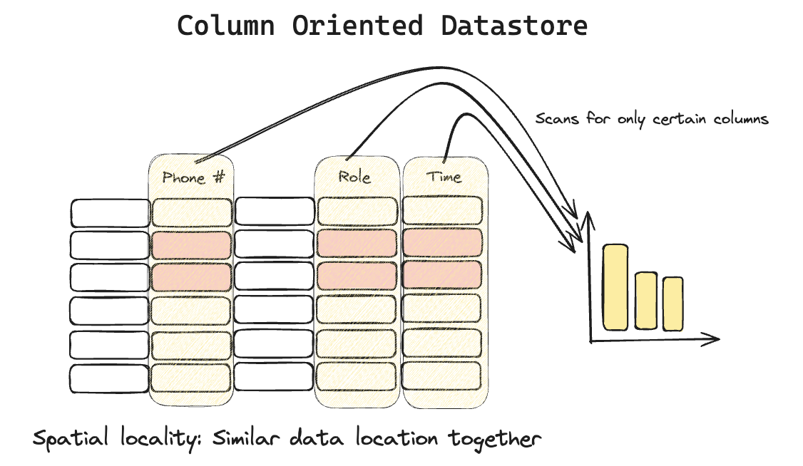
Column-Oriented Store
Same data is stored as columns at storage layer.
For example
|ID| Name | Department |Role|
|10|Ram   | Devops     |SDE1|
|20|Sam   | Security   |SDE2|
|30|Aditi |Software Dev|SDE3|
In a OLAP DB, queries are mostly related to columns, like show me the list of users whose salary is >$1000 who belong to the SDE2 role. Here, it makes sense to store data in columns so that the GROUPBY clauses are more efficient.
Efficiency in Column-oriented
- COMPRESSION
It is easier to compress data in column-oriented data as similar data (Columns) are stored nearby. For example, if timestamp is present in column; a run-length encoded scheme can be used where the first timestamp can be stored as a Unix timestamp; whilst the rest of data can be stored as increment. This was lower the space cost as increments can be stored in less number of bits.
- Late Matrialization
As data is located in separate places, the data is formed at the end as a lot of combining of columns takes place at later stage.
For aggregate, using Column-store makes more sense as a lot of unnecessary columns can be read in row-stores which are discarded in the query execution cycle.
All big data formats are looking into storing data in column stores.
Examples for column-oriented file formats:
Apache Arrow: Store data in columnar data memory format
Apache Parquet: Column-oriented data format for efficient data storage and retrieval
Apache ORC: Columnar storage for Hadoop database
And examples for column-oriented data stores:
Clickhouse: Storing databases in column
DuckDB: Columnar-vectorized query execution engine
OLAP over the decades
1990s - 1st first generation OLAPs - DATA CUBES
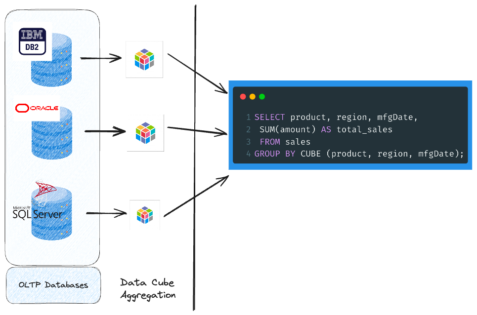
Here the data from disparate sources are fetched and combined into a data cube.
These are then aggregated which can then be queried for analyitcal purposes.
But this was created in the 1990s, where the data was simple and less granular than we have today. Now we have all sorts of data with varying types present in our databases. The simple Employee database with simple columns no longer exist. Hence, it lead to poor scalability and flexibility.
Also, since data sources were from different sources, it lead to higher data duplication which in turn lead to higher data storage costs.
Examples:
| Tool | Note |
| MSFT SQL Server | Data Cube |
| Oracle | Data Cube |
| Terradata | OLAP from day1 |
| Sysbase | Data Cube |
| IBM DB2 | Data Cube |
| Informateica |
2000s - Second Generation Architectures
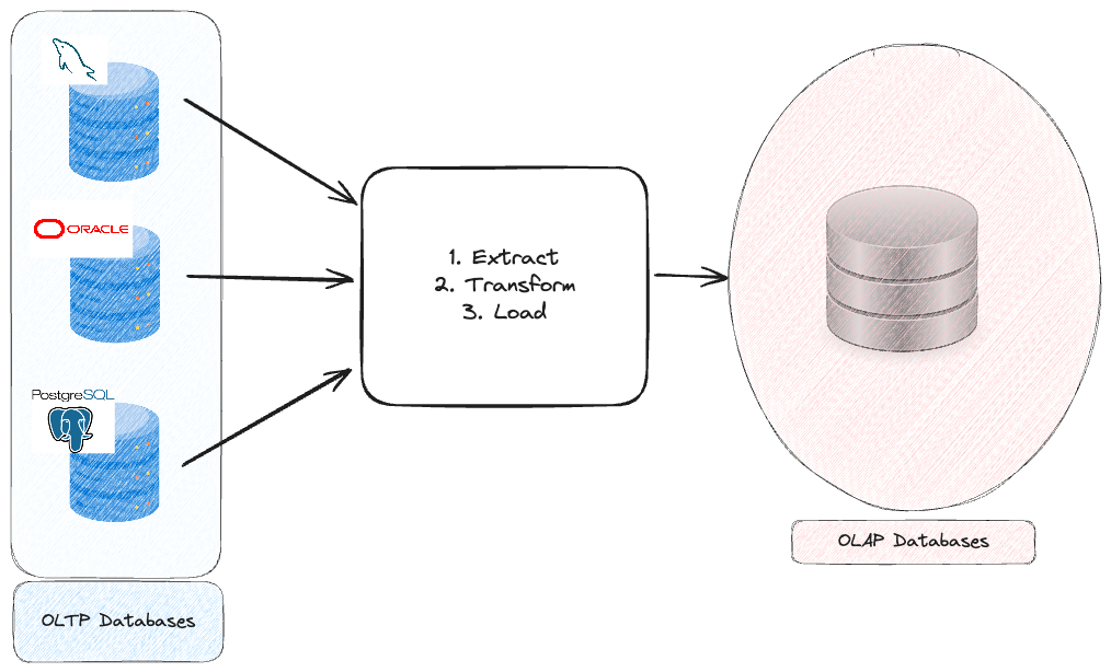
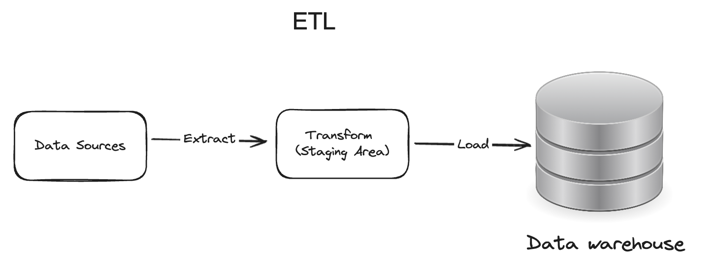
In 2000s, there was a new paradigm of ETL (Extract, Transform, Load)
Extract: Pull raw data from multiple sources. This could be databases, CSVs, JSON etc
Transform: Transform data to be dumped to OLAP database. Transformation could be cleaning data, creating proper data model as per business need etc
Load: Load into a database which can be consumed by business via tools such as PowerBI, Tableau, DOMO etc.
A lot of Data-warehouse came into picture such as MonetDB, Vermica.
A hidden fact is most of these data-warehosues were forks of traditional Databases which were modified to improved coulmn-oriented analytical queries. This was discussed at Improving Row-oriented datastore to become Column-oriented section
Examples:
| DB | Note |
| Netezza | Forks of Potgres |
| ParAccel | Forks of Potgres |
| MonetDB | Duckdb v1 was based on MonetDB. V2 is not MonetDb |
| Greenplum | Forks of Potgres |
| DataAllegro | Microsoft bought |
| Vertica | Fork of Potgres |
2010s and now: Rise of Decoupled OLAPs
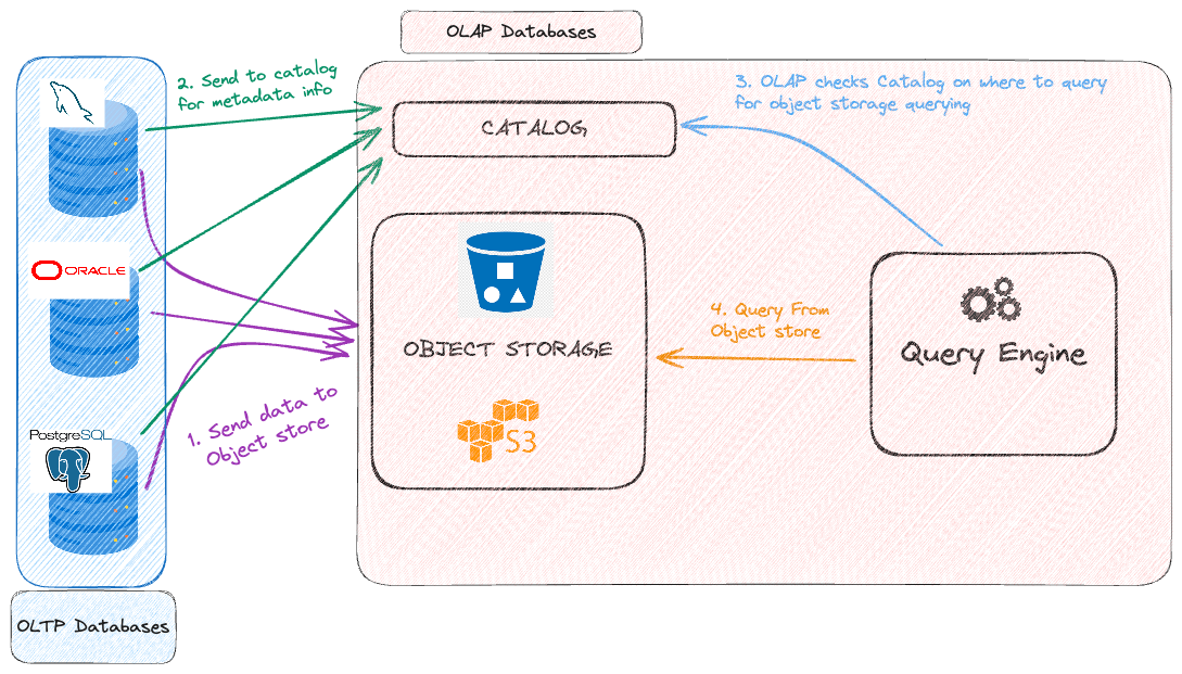
Send Data to a decoupled Object Storage
Send Metadata information to a catalog/metadata store
Query Engines queries the catalog/metadata store to get the location and other information on how to query data.
Query Engine queries the object storage and pulls data.
Processes the data based on filtering criteria and sends result to client.
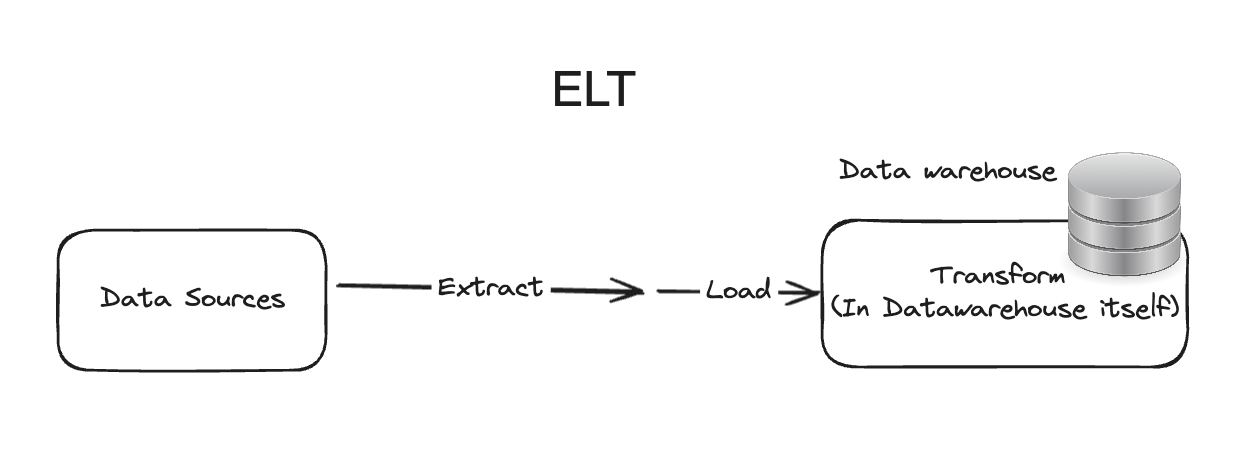
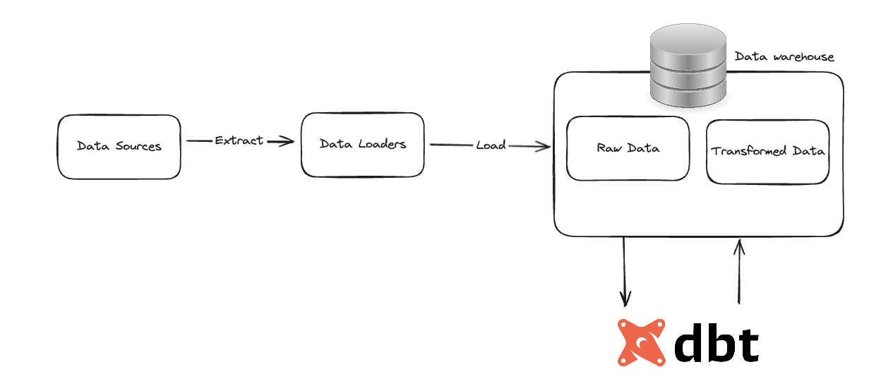
Modern OLAP has moved away from traditional ETL workflow to a ELT workflow, where the transform step happens alter load. dbt is one of the technologies that leverages ELT to transform data immediately after extracting.
Examples:
| DB | What | Integration |
| Hive | DW system which is used with Hive-metastore. Not ideal for object storage which is part of modern OLAP | Integrates with Hadoop such as HDFS, Pig etc |
| Apache Drill | Schema-less Query engine for Hadoop, NoSQL and Cloud storage | Integrates with Hadoop ecusystem |
| Duckdb | In-porcess OLAP | Supports various file format such as CSV, Parquet JSON etc |
| Druid | Real-time analytics DB for batch and streaming data | Streaming such as Kafka |
| Presto | SQL query engine by Facebook | Integrate with various file format, OLAP DBs and visualisation tools |
| Snowflake | Written from groundup and is a whole platform for data engineering including hosting, querying, RBAC etc | Integrates with everything |
| Pinot | Realtime distributed OLAP datastore from Linkedin | Integrates with Kafka, S3, Tableau, Presto etc |
| Redshift | Built on top of ParAccel | Integrates nicely with AWS ecosystem |
| Apacka Spark | Data analytics engine to do high-volume data processing | Integrate with object stores etc |
| Google Bigquery | Google's OLAP | Integrate with GCP |
ETL vs ELT and the DBT Approach
1. ETL
The three phases as discussed in the 2000s database section can be represented here:
- ELT
- DBT: Implementing ELT in real-world
Advantages of ELT vs ETL
Versioned Control workflows: As in ELT; data transformation requires a feedback with data load; it is possible to allow VCS and CI/CD workflows on the data which is a common practice in Software engineering and Agile teams
Faster feedback loop: As data is transformed on the fly, we can get a better feedback on insights from data, instead of waiting for a cron job that executes the data dump into datawarehouse.
Push vs Pull between Data & Query
There are a couple of ways to execute query in OLAP ecosystem. These are
Push Query to Data
Pull Data to Query
1.Push Query to Data
In the earlier days, networking and data fetching was slow and expensive. So idea was to send query directly to the OLAP database system. Then data (based on executed Query) was sent back to client over the network.
2.Pull Data to Query
Now we have modern OLAP with Shared-Disk architecture where the compute cannot be possible in shared-disk-not-compute architecture. Also, the network and data fetching (thanks to SSDs) speeds have improved. This allows of moving the data to the query engine(as discussed earlier) for processing.
Modern OLAP does the combination of 1. and 2. in context of what type of dat a workload, how frequent data are accessed (available via data querying statistics); decisions are made whether to bring query to data; or data to query.
Conclusion
Hope you learned the need of OLAP databases and why there has been a degree of change for every decade in the OLAP world.
The following the references without which this could not have been possible:
References
-
Paper Link: Column-Stores vs. Row-Stores: How Different Are They Really?


